Geometry tutorial

Bramble.jl provides a high-performance, zero-allocation geometric modeling subsystem designed for partial differential equations (PDEs) and numerical discretization schemes on Cartesian and tensor-product meshes.

In this tutorial, you will learn how to:

1. Construct 1D intervals and multi-dimensional CartesianProducts.
2. Handle collapsed (lower-dimensional) geometries.
3. Query spatial and topological dimensions, bounds, centers, and containment.
4. Define boundary labels and markers with markers.
5. Build complete computational Domains ready for mesh generation and PDE solvers.

1. Sets and intervals

At the core of the geometry system is CartesianProduct{D, T}, which represents the Cartesian product of $D$ closed intervals in $\mathbb{R}^D$ with coordinate type T.

1.1 Creating 1D intervals

Use interval to define closed intervals $[a, b] \subset \mathbb{R}$:

using Bramble

# Define the interval [0.0, 1.0]
I = interval(0.0, 1.0)

# Automatic conversion of integer bounds to floating point
I_int = interval(0, 2)  # CartesianProduct{1, Float64}

# Create a single degenerate point [0.5, 0.5]
P = point(0.5)

# Bounding box of any two numbers (ordered automatically)
B = box(1.5, 0.2)       # [0.2, 1.5]

1.2 Multi-dimensional sets via the tensor product operator ×

Multi-dimensional hyper-rectangles are constructed intuitively by taking the tensor product of lower-dimensional sets using the × (\times<tab>) operator:

# 2D Unit square: [0, 1] × [0, 1]
Ω_2d = interval(0.0, 1.0) × interval(0.0, 1.0)

# 3D Cuboid: [-1, 1] × [0, 2] × [0, 0.5]
Ω_3d = interval(-1.0, 1.0) × interval(0.0, 2.0) × interval(0.0, 0.5)

2. Querying geometric properties

Bramble.jl provides a type-stable interface for querying geometric properties:

X = interval(0.0, 2.0) × interval(-1.0, 1.0)

# Spatial embedding dimension (D = 2)
dim(X)            # 2

# Topological dimension
topo_dim(X)       # 2

# Interval bounds
extrema(X)          # ((0.0, 2.0), (-1.0, 1.0))
extrema(X, 1)       # (0.0, 2.0)  -- bounds in dimension 1
extrema(X, 2)       # (-1.0, 1.0) -- bounds in dimension 2

# Geometric center
center(X)         # (1.0, 0.0)

# 1D projection onto a specific axis
proj_x = projection(X, 1)  # interval(0.0, 2.0)

Point containment

Check whether a point lies within a CartesianProduct:

# In 1D:
I = interval(0.0, 1.0)
0.5 ∈ I           # true
1.5 ∈ I           # false

# In 2D (supports Tuples, SVector, and Vectors):
X = interval(0.0, 1.0) × interval(0.0, 1.0)
(0.5, 0.5) ∈ X    # true
(1.2, 0.3) ∈ X    # false

3. Collapsed and lower-dimensional geometries

A dimension is considered collapsed when its interval is degenerate ($a = b$). Bramble tracks collapsed dimensions without heap allocations, so a lower-dimensional surface or interface embedded in a higher-dimensional space can be modeled directly:

# 1D line embedded in 2D space: x ∈ [0, 1], y = 0
line_in_2d = interval(0.0, 1.0) × point(0.0)

dim(line_in_2d)       # 2 (spatial embedding dimension)
topo_dim(line_in_2d)  # 1 (topological dimension)

# Check if individual dimensions are collapsed
line_in_2d.collapsed[1]  # false (x-axis is extended)
line_in_2d.collapsed[2]  # true  (y-axis is collapsed)

4. Boundary markers

PDE boundary conditions require tagging specific domain boundaries (e.g., Dirichlet, Neumann, Robin, inflow/outflow).

4.1 Boundary symbol conventions

Bramble provides canonical coordinate-aligned boundary symbols across all dimensions to eliminate axis transposition ambiguities in multi-dimensional physics simulations:

• 1D: :xmin (:left), :xmax (:right)
• 2D: :xmin (:left), :xmax (:right), :ymin (:bottom), :ymax (:top)
• 3D: :xmin (:back), :xmax (:front), :ymin (:left), :ymax (:right), :zmin (:bottom), :zmax (:top)

Camera- and viewpoint-dependent labels (:left, :right, :bottom, :top, :front, :back) remain supported as 100% backward-compatible aliases.

You can inspect standard boundary symbols using boundary_symbols:

boundary_symbols(2)
# (:xmin, :xmax, :ymin, :ymax)

4.2 Creating markers

Markers are defined as :label => identifier pairs where identifier can be a single boundary symbol, a tuple of symbols, or a boolean function:

geom = interval(0.0, 5.0) × interval(0.0, 1.0)

# 1. Using the markers() constructor
# Define markers using pairs of :label => boundary_spec
m1 = markers(
    geom,
    :inflow  => :left,
    :outflow => :right,
    :wall    => (:top, :bottom)
)

# Retrieve all defined labels
collect(labels(m1))
# [:inflow, :outflow, :wall]

4.3 Function-based and time-dependent markers

You can also define internal or geometric subset markers using boolean condition functions, as well as time-dependent markers:

# Condition-based marker: tag a subsection of the boundary or domain
m_cond = markers(
    geom,
    :inflow    => :left,
    :hot_spot  => (p -> p[1] > 2.5 && p[2] ≈ 0.0)
)

# Time-dependent markers:
time_span = interval(0.0, 10.0)
m_time = markers(
    geom,
    time_span,
    :moving_source => ((p, t) -> norm(p .- [t, 0.5]) < 0.2)
)

# Evaluate time-dependent markers at time t = 1.5
m_evaluated = m_time(1.5)

5. Computational domains

A Domain joins a geometric set (CartesianProduct) with its boundary markers into a single unified object:

# 1. Define geometry
geom = interval(0.0, 1.0) × interval(0.0, 1.0)

# 2. Construct domain with inline boundary markers
Ω = domain(
    geom,
    :dirichlet => (:left, :right),
    :neumann   => (:top, :bottom)
)

# Or create a default domain marking all external boundaries as :boundary
Ω_default = domain(geom)

5.1 Domain traits

Domain automatically delegates geometric and marker methods directly:

dim(Ω)            # 2
topo_dim(Ω)       # 2
extrema(Ω)        # ((0.0, 1.0), (0.0, 1.0))
center(Ω)         # (0.5, 0.5)
(0.5, 0.5) ∈ Ω    # true
Bramble.is_collapsed(Ω)    # false (checks if any dimension is degenerate)
Bramble.is_collapsed(Ω, 1) # false (checks dimension 1)

# Access underlying set and markers — `set` and `is_collapsed` are `public`, not exported, so they use `Bramble.`
Bramble.set(Ω)    # CartesianProduct{2, Float64}
markers(Ω)        # DomainMarkers
collect(labels(Ω)) # [:dirichlet, :neumann]

Iterating directly over label_symbols(Ω), label_tuples(Ω), or label_conditions(Ω) allocates 0 bytes.

6. Practical examples

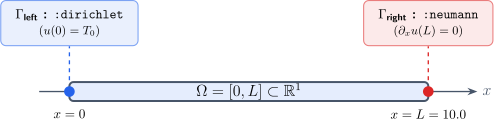
Example 1: 1D rod with mixed boundary conditions

Consider heat conduction along a 1D rod $\Omega = [0, L]$ with $L = 10.0$, fixed temperature at $x = 0$ (:left) and insulated end at $x = L$ (:right):

L = 10.0
rod_geom = interval(0.0, L)

# Define domain with Dirichlet left boundary and Neumann right boundary
rod = domain(
    rod_geom,
    :dirichlet => :left,
    :neumann   => :right
)

println("Domain: ", rod)
println("Dimension: ", dim(rod))
println("Active Labels: ", collect(labels(rod)))

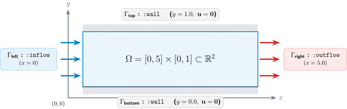
Example 2: 2D channel flow domain

Consider fluid flow in a rectangular channel $[0, 5] \times [0, 1]$ with an inflow on the left, outflow on the right, and no-slip walls on top and bottom:

channel_geom = interval(0.0, 5.0) × interval(0.0, 1.0)

channel = domain(
    channel_geom,
    :inflow  => :left,
    :outflow => :right,
    :wall    => (:top, :bottom)
)

@assert dim(channel) == 2
@assert (2.5, 0.5) ∈ channel
println("Channel labels: ", collect(labels(channel)))

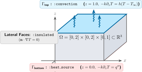
Example 3: 3D heat sink domain

Consider heat dissipation across a 3D block $[0, 2] \times [0, 2] \times [0, 1]$ subjected to a bottom heat source, top convective cooling, and insulated lateral walls:

sink_geom = interval(0.0, 2.0) × interval(0.0, 2.0) × interval(0.0, 1.0)

sink = domain(
    sink_geom,
    :heat_source => :zmin,  # or legacy alias :bottom
    :convection  => :zmax,  # or legacy alias :top
    :insulated   => (:xmin, :xmax, :ymin, :ymax)  # or (:left, :right, :front, :back)
)

println("3D Domain Center: ", center(sink))
println("Active Labels: ", collect(labels(sink)))